Day 3: Importing needed libraries, Importing the dataset and printing it out
Python Libraries
Copy code to the clipboard.
Click on Start.
Click on Anaconda 3 64 bit
Select Jupyter Notebook Anaconda 3.
Select New.
Select Python 3.
Click on the first frame.
Press CTRL V to paste text into python.
Click on file and save it as storeClosures.ipynb
Click Run to run first frame.
Getting the dataset and pasting code into Python
In Python, click on the + sign to insert a cell below.
Paste your code in that cell.
You will have to modify the folder location for your files.
The two reverse slashes are very important in the code. Make sure that you use them.
Run your code for the first two cells.
Your screen should look like this.
What does this part of the program show us? First the shape of the dataframe is displayed (100,7). We have 100 entries in the file and it is arranged in 7 diferent columns.
Next the entire dataframe is printed out.
df.print info prints a description of the dataset.
The last line prints Original DataFrame.
Day 4: Splitting the data into features and labels
In Python, click on the + sign to insert a cell below.
Paste your code in that cell.
The features are the input data: Income, Cash flow, new customers, customer satisfaction and employee performance numbers,
The labels are the the yes and no responses as to store closures.
Save your program.
Day4 : Training the algorithum to solve the classification problem.
In Python, click on the + sign to insert a cell below.
Paste your code in that cell.
Save and Run your program. Here is what the output looks like.
Random Forest’s ensemble of trees outputs either the mode or mean of the individual trees.
This method allows for more accurate and stable results by relying on a multitude of trees rather than a single decision tree.
The reasoning behind the Random Forest model is that individual decision trees perform much better as a group than they do alone.
When using Random Forest for classification, each tree gives a classification or a “vote.”
The forest chooses the classification with the majority of the “votes.”
The n_estimators line determines the number of trees in the forest. One hundred is the default. We set ours to 20
The test-size variable determines the size of the random sample. In our case, it is 20 out of 100 in the dataset.
That is why there are 20 predictions.
The random_state = 0 makes it so that it replicates the same set of random numbers each time it is run.
If you remove that piece of code, you will get a different set of prediction samples each time you run the program.
Analysis of the data
The predictions appear at the bottom of the list. They are the y's and n's.
The first prediction is for Store 26, which is az7. Our model says that based on the data. that store should remain open. The original data agrees with the prediction. This would be a true positve on the confusion matrix.
The last preciction is a 'n' for 8 which is store ca9. Both actual and predictions are a "n" for this store. This wouuld be a true negative on the confusion matrix.
Day 5: Accuracy of the model
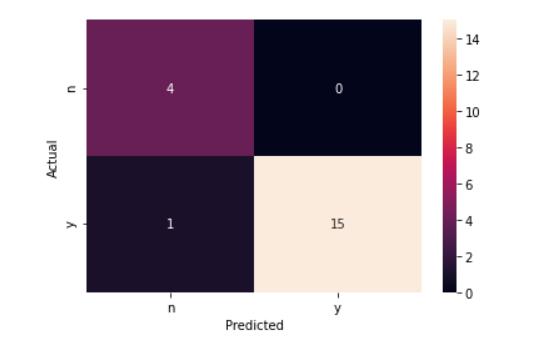
A confusion matrix is a graphical presentation showing the performance of our model.
The true negatives, TN are ones where the actual and predictions were both false "n". In the random sample, there were 4 of these.
The true positives, TP are the ones that the actual and predictions were both true. In our random sample, there were a total of 15.
The false positives, FP are the ones where the actual was false and the prediction was true. Our model did not generate any of these.
The false negatives, FN are the ones where the actual answers were true and the predictions were false. We had one of these n our random sample.
Let's see if we can find this false negative.
I looked through the data set and the predictions. array item 2, ca3 in the actual data was "y" and the prediction was "n"
When counting the y, and n at the bottom of the prediction list, start counting starting with 0.
The accuracy percent for our model is calculated as follows (TN + TP)/(TN + TP + FP + FN + FP ) or (4 + 15)/(4 + 15 + 1 + 0) = .95
There is a line in our code, that allows you to enter one stores' data and have it predict whether to keep the store open or close it.
prediction = clf.predict([[.01,100,1,1,1]])
If you enter these numbers, you will find that this store should be closed.
Try some different numbers. This line is especially useful.
The last section of code tells us which of the factors are the most important when deciding store closures.
The predictions show the following results.
4 0.566881 Employee Performance
0 0.187552 Net Profit
1 0.166781 Cash Flow
2 0.042852 New Customers
3 0.035935 Customer Satisfication
A working predictive model needs to make predictions for data that it hasn't seen yet.
We are assuming that next year's results will imitate the predictions above.
As you can see from the results, The biggest reason a store got a "n" response for save store was based on poor employee evaluations: .566881
Customer satisfaction, array number 3 had the least importance, 0.035935.
Number of new customers was also not seen as not very important with a score or 0.042852
Net profit and cash flow scores fell in the middle of items of importance.
Action Plan
As result from our research we conclude that failing stores, those with a "n" for save store column are failing mainly due to poor employee performance.
First find out which department in the failing stores has the problem with employee performance evaluations. It could be the stores' management teams, sales force, etc.
We should recommend to the corporate top management that there either needs to be a major inservice for those employees with numbers below average, 4.94 out of 10 or they should be terminated and management should hire new employees.
The numbers for net profit and cash flow are accounting data predictions.
Both net profit and cash flow can be improved by increasing sales at these stores.
Sales
- Cost of goods sold
= Gross Profit
- Total operating expenses
= Net profit
Sales can be increased by in-store displays of profitable merchandise. Advertising can be increased. Customer loyality programs could be initiated. Retrain the sales force.
Expenses can also be reduced. Examine cost of good sold, insurance, utlities and labor costs.