In this lesson, you will learn about "outliers". In datasets there can be values too far away from most of the rest of the observations. For example if the height of a person is between 60 and 80 inches, then 96 inches would be an outliner since such an observation occurs rarely. Outliers can distort your statistical model's results. There a number of ways to deal with outliers. We will examine the first two of them.

Remove the outlier from the dataset: trimming
Cap the outliers and replace them using mean and standard deviation
Treat the outliers are missing values
Include the outlier along with the other data points at the tail

A Box Plot is a good way to visualize an outlier. In descriptive statistics, a box plot or boxplot is a method for graphically demonstrating the locality, spread and skewness groups of numerical data through their quartiles.[1] In addition to the box on a box plot, there can be lines (which are called whiskers) extending from the box indicating variability outside the upper and lower quartiles, thus, the plot is also termed as the box-and-whisker plot and the box-and-whisker diagram.¹

The dataset that we will be working with has to do with a food truck, stationed at different locations during the week. Location, Number of meals, time of day and revenue data have been entered into a spreadsheet and we will be looking at the csv file.

Day 1: Python Libraries, and examining the dataset and removing outliers, (trimming).

First get a copy of the file.

Outliers File

Open a new Python project, click copy text button and paste the contents into the first frame.

You will have to adjust the location of the file.

Run the code in the first frame.

This code imports libraries from Python, loads the dataset and prints it's shape and head

Create a new frame and key in the following: foodTruck_data = dataset

Create another new frame and key in the following code:print(dataset.describe())

Save and run the first three frames. You should see the dataset described.

You can see that max number of meals is 200, an outlier. The mean is 2.74 and the standard deviation is 7.5.

Now we need to define the variables. We believe that this statistical model is a linear one since the more meals ordered, the more revenue will be generated.

Create a new frame, click copy text button and paste the contents into the frame.

Run the code for all frames.

Create a new frame, click copy text button and paste the contents into the frame.

Run the code for all frames.

Output for this frame should look like the data below.

Coefficient
Location 0.437376
Num_Meals 19.668538
Time 0.010477

For every one-unit increase in [X variable], the [y variable] increases by [coefficient] when all other variables are held constant.

For every additional meal sold, revenue will increase by $19.67.

Now let's see predictions of the model. Use the following code.

Create a new frame, click copy text button and paste the contents into the frame.

Run the code for all frames.

Output for this frame should look like the data below.

Day 2: Predictions and Finding Outliers

Our model did not do a very good job in predicting revenue. We have to consider that outliers, number of meals sold were more that our 1-4 normally sold.

For example, record 150, 152 in the spreadsheet, the actual revenue was $60.25. Our model predicts $80 for the revenue. That is a large discrepancy. Let's look at some metrics for model errors. Use the following code.

from sklearn import metrics
print('RMSE:', np.sqrt(metrics.mean_squared_error(y_test, pred_y)))
You should get the following output.
RMSE: 9.856476253257808

Low RMSE values indicate that the model fits the data well and has more precise predictions. Conversely, higher values suggest more error and less precise predictions.

One way to assess how well a regression model fits a dataset is to calculate the root mean square error, which is a metric that tells us the average distance between the predicted values from the model and the actual values in the dataset.²

Our calculated RMSE is $9.85. That means our predictions differ $9.85 from actual amounts.

We really can't use this model for predicting future revenue. We need to see what caused the large discrepancy.

If we have any outliers that could throw off our precictions. That is what we are going to do in the next section

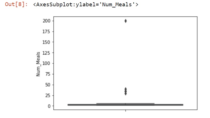
A good way to see outliers is by using a box plot.

Create a new frame, click copy text button and paste the contents into the frame.

Run the code for all frames.

Output for this frame should look like the data below.

The box plot shows us that most of the meals sold are between 1 and 5.

The graph also shows the outliers. They are the black dots. There are some between 25 and 50 and one at 200. These items can negatively affect our statistical model. We need to deal with these outliers to create a better model.

One of the most used way to remove them is to find the Inter Quartile Range (IQR). Multiply it by 1.5 and then subtract it from the first quartile value (.25) to find the lower limit. To find the upper limit, add the product of IQR and 1.5 to the 3rd quartile value, (.75).

IQR can be calculated subtracting the first quartile value from the 4^th quartile.³

Day 3: Trimming the outliers

Outlier trimming means that we are going to remove outliers beyond a certain threshold value. We are going to remove outliers from the number of meals column. These large number of meals were for catering events and do not give us a clear picture of our day to day revenue.

Create a new frame, click copy text button and paste the contents into the frame.

Run the code for all frames.

Output for this frame should look like the data below.

-2.0
6.0
Any outlier(number of meals) less that -2 or over 6 need to be eliminated

Now we need find the rows containing those oulier values.

Create a new frame, click copy text button and paste the contents into the frame.

There is no output from this code.

Create a new frame, click copy text button and paste the contents into the frame.

There is no output from this code.

Now let's see how many rows were eliminated. Create a new frame and key in this code.

foodTruck_data.shape,foodTruck_without_Num_Meals_outliers.shape

The ouput should look like:

((776, 4), (771, 4))

This shows that the original data set contained 776 rows and 4 columns. The new dataset after eliminating the outliers shows 771 rows and 4 columns. We eliminated 5 rows (776-771).

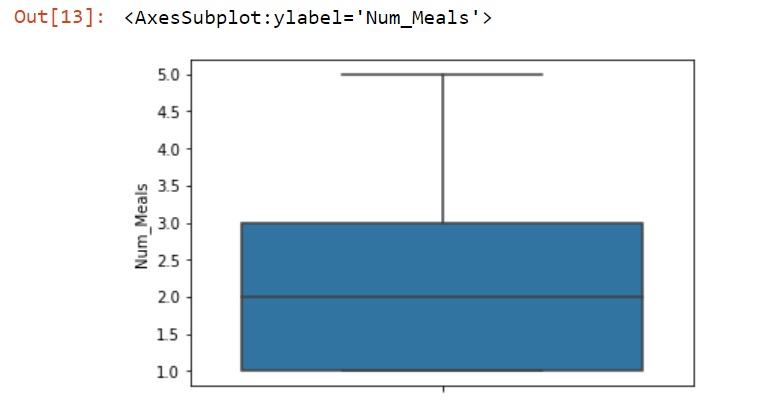
Now we are going to plot a box plot to verify that the outliers have been eliminated before we begin to train the model.

Create a new frame and key in the following code.

sns.boxplot(y = 'Num_Meals',data = foodTruck_without_Num_Meals_outliers)

Your output should look like the image below.

You can see from the box plot that there are no more outliers.

Create a new frame, click copy text button and paste the contents into the frame.

These lines of code sets new variables for X and y after eliminating the rows containing outliers.

There is no output from this line of code.

Create a new frame, click copy text button and paste the contents into the frame.

Save and run all frames.

You should get the following output.

Coefficient
Location -0.039951
Num_Meals 12.128038
Time -0.000256

Now we can predict that for every additional meal sold, revenue will increase by $12.12. Remember that this number was $19.67 before eliminating the outliers.

Next, we need to see individual predictions.

Create a new frame, click copy text button and paste the contents into the frame.

Save and run all frames.

You should get the following output.

Look at how much closer the predictions are to the actual amounts compared to the predictions that included the outliers.

The last step for this model is to look at the RSME amount.

Create a new frame and key in the folloing lines of code.

from sklearn import metrics
print('RMSE:', np.sqrt(metrics.mean_squared_error(y_test, pred_y)))

The output from these two lines should look like:

RMSE: 0.45942996024679505

Look how much lower this RMSE is compared to the RMSE before trimming the outliers.

We can conclude that this is a good statistical model for predicting future revenues for our food truck business.

Day 4:Outliner Capping Using Mean and Standard Deviation

Upper and lower limits for outliners can be calculated using the mean and standard deviation method.

If you did not get a copy of the file , do so here and save it your computer as a ,csv file.

Outliers File

Create a new project, click copy text button and paste the contents into the frame.

Adjust where your file is located.

Save and run the frame.

You should get the following output.

Now we are going to make a box plot graph to find out outliers.

Create a new frame, click copy text button and paste the contents into the frame.

Save and run the frame.

You should get the following output.

As in the outlier trimming section of this lesson, you should get the same result. There are a number of outliers clustered between 25 and 50 and one at 200.

Now we need to get the upper and lower limits as to revenue amounts to eliminate the outliers.

Create a new frame, click copy text button and paste the contents into the frame.

Save and run the frame.

You should get the following output.

-19.957164118057072
25.43912288094367

This outlier method uses the mean and standard deviation to calculate these numbers, whereas the trimming method, just eliminates these outliers, consequently the numbers for high and low limits differ greatly.

Now we are going to replace the outliers.

Create a new frame, click copy text button and paste the contents into the frame.

Save and run the frame.

There is no output.

Now, let's make a box plot to see if out outliers have been replaced.

Key in the following code in a new frame.

sns.boxplot(y ="Num_Meals", data = foodTruck_data)

Save and run. You should get the following output.

Create a new frame, click copy text button and paste the contents into the frame.

Save and run the frame.

Your output should look like this.

The original mumber of meals for the first row was 30. You can now see that it was replaced with 25, which is the mean.

Let's see if all the outliers were replaced. Key in the code below to check.

Create a new frame, click copy text button and paste the contents into the frame.

Save and run the frame.

Your output should look like this.

Create a new frame, click copy text button and paste the contents into the frame.

Save and run the frame.

There is no output. We are assigning variable for x and y

Now it is time to train the model.

Create a new frame, click copy text button and paste the contents into the frame.

Save and run the frame.

Your output should look like this.

Coefficient
Location 5.456836
Num_Meals 45.995891
Time 0.065378

The number of meals is the most important variable when determining revenue.

Create a new frame, click copy text button and paste the contents into the frame.

Save and run the frame.

Your output should look like this.

As you can see the actual numbers and predictions differ greatly. This model is not a good one for making revenue predictions using the mean for outliers.

Let's look a the RMSE score. Create a new frame and key in the following lines.

from sklearn import metrics
print('RMSE:', np.sqrt(metrics.mean_squared_error(y_test, pred_y)))

You should get the following result.

RMSE: 50.16919899620588

Compare this number to the RMSE for the outlier trimming program.